Sorting
Now that we can judge the algorithmic complexity of code, it's time to look at a very common and applicable subject in computing: sorting!
Sorting involves the act of ordering items in a collection systematically.
The systematic aspect of sorting has been of research interest for computer scientists since the dawn of the digital age, and many algorithms have sprung forth from such endeavors.
Just as we know that not all algorithms were created equal, so must we observe that not all sorting methods are equally good for certain sorting tasks.
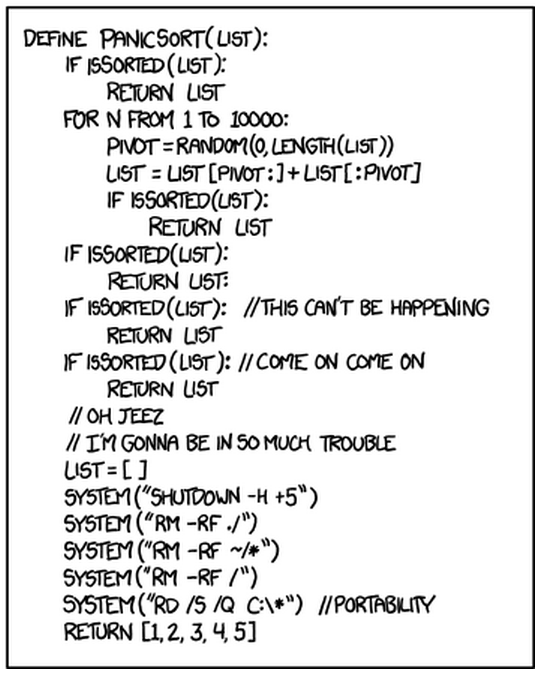
We'll now examine several sorting algorithms, see how they work, what they're good at, and what they're horrible at, all to avoid producing sorting algorithms like the following:
Quadratic Sorts
The quadratic sorts are those that perform with O(n^2) time complexity... they're not that great, and there's rarely a good reason to use them.
Now let's study a couple :)
Bubble Sort
Perhaps the cliche first-sorting-lesson algorithm, bubble sort operates with the following steps:
  for each item i in the array of n items:
      for each item j from n to i+1:
          if the item at a[j] is less than the item at a[j-1]
              swap those two items
      stop if you didn't swap any items on this iteration
So essentially, just compare two adjacent numbers from the back to the front of the array, arranging the two with the lesser on the left and greater on the right (assuming ascending order), and continue to do so until the smallest numbers have "bubbled" to the front, and the largest have bubbled to the back.
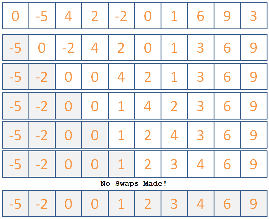
Use Bubblesort to sort the following list of ints:
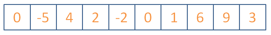
Click here for the steps the algorithm would take.
Now that we've seen how it's done, let's look at how to implement it in code:
Complete the shell for BubbleSort described below:
  // Helper to print out array elements
  void printIntArr (int arr[], int size) {
      for (int i = 0; i < size; i++) {
          cout << arr[i] << " ";
      }
      cout << endl;
  }

  // Helper function; swaps two array elements via
  // the input pointers
  void swapInts (int* i1, int* i2) {
      int temp = *i1;
      *i1 = *i2;
      *i2 = temp;
  }

  // Not to be confused with BubleSort, which
  // just replaces your array elements with lyrics
  // from Haven't Met You Yet
  void bubbleSort (int arr[], int size) {
      // [!] Iterate through each element of the
      // list
      for ( ??? ) {
          // Track if a swap has been made
          bool swapped = false;
          // [!] Iterate through all elements of the list
          // starting at the end element and up to the
          // i + 1 element
          for ( ??? ) {
              // [!] Swap if the two currently adjacent
              // in the 2nd loop iteration are out of order
              if ( ??? ) {
                  swapInts( ??? );
                  // Mark that you've swapped
                  swapped = true;
              }
          }
          // [!] Return if you made no swaps
          if (!swapped) {return;}
      }
  }

  int main () {
      int i[] = {0, -5, 4, 2, -2, 0, 1, 6, 9, 3};
      bubbleSort(i, 10);
      printIntArr(i, 10);
  }
Bubble sort can "sort" a list in linear time if the list has what property?
It's already almost sorted :P
What list property will cause BubbleSort the most inconvenience?
Reversed order of elements.
There are some good BubbleSort animations located here.
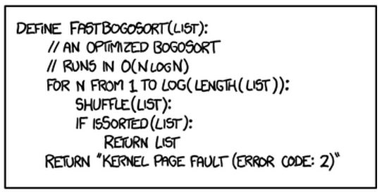
OK nice! Got a simple sort down... here's another one that you should avoid writing on a midterm:
Insertion Sort
The second most cliche sorting algorithm, insertion sort operates with the following steps:
  for each element i in the array, starting with the 2nd:
      for each element k = i down to k = 0 where arr[k] < arr[k-1]:
          swap a[k] and a[k-1]
So, the idea is that we continue to lock items at the front of the array into their proper place, assuming everything to the left of the current one is sorted already.
Use Insertion Sort to sort the following list of ints:
Click here for the steps the algorithm would take.
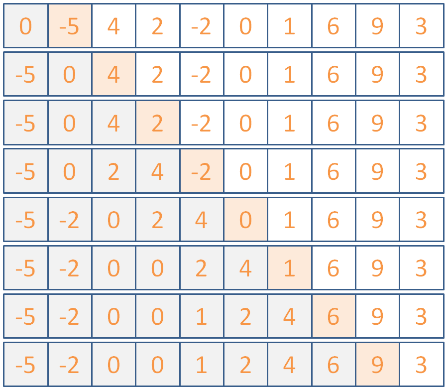
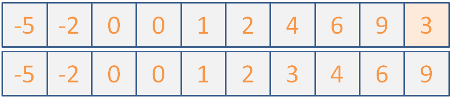
(maybe if I don't say anything, they won't notice that the illustration is actually two different images because I couldn't fit it all into one slide...)
Any who, let's implement this now; it won't take long!
Implement the insertionSort skeleton begun below.
  void insertionSort (int arr[], int size) {
      // [!] Iterate through each element of the array
      // starting with the second
      for ( ??? ) {
          // [!] Iterate through the first i elements
          // of the array, except the first
          for ( ??? ) {
              // [!] If the currently examined
              // element is greater than the one
              // before it in the list, stop
              if ( ??? ) {
                  break;
              }
              // [!] Otherwise, swap the two
              swapInts( ??? );
          }
      }
  }
Insertion sort can "sort" a list in linear time if the list has what property?
It's already almost sorted... same as BubbleSort, but insertion sort has less overhead
What list property will cause Insertion Sort the most inconvenience?
Reversed order of elements.
There are some good Insertion animations located here.
I think that's it for covering quadratic sorts... remember that these have O(n^2) and are generally not preferred on their own in the general case.
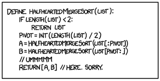
Let's take a quick review of merge sort, unlike the following half-hearted implementation:
Better Sort Algorithms
We can do much better than quadratic sorting time; let's look at some alternatives below:
Merge Sort
Merge sort is a recursive algorithm that performs the following three steps in the example code below (note: the merge function is a bit complicated for this example, so it exists only in name below):
  void mergeSort (int a[], int b, int e) {
      if (e - b >= 2) {
          int mid = (b + e) / 2;

          // Recursive call on first half of a
          mergeSort(a, b, mid);
          // Recursive call on other half of a
          mergeSort(a, mid, e);

          // Merge those sorted subpropblems!
          merge(a, b, mid, e);
      }
  }

  int main () {
      int arr[] = {4, 3, 1, 2};
      sort(arr, 0, 4);
      // arr will now be {1, 2, 3, 4}
  }
Here, the merge function combines the two sublists into a single, ordered sublist.
Let's take another look at it in action (gif shamelessly stolen from Wikipedia):
What is the time complexity of MergeSort?
O(n*log(n)) because it continuously splits the array into smaller subarrays [O(log(n))], and then merges them [O(n)]
Taking into account its splitting and merging behavior, are there any properties of lists that MergeSort struggles with?
MergeSort actually handles input of any type pretty much the same; because of the splits down to small, managable sub-arrays, the format of the larger array is not relevant to its performance.
There are some good MergeSort animations located here.
Quick Sort
The sort of choice for the discerning programmer, Quick Sort (or some variant of it) is used in many modern sorting applications.
It goes something like this:
  Return the current array if 1 element or fewer
  Randomly choose a pivot value in the array
  Remove the pivot from the array
  For each remaining array element:
      Put those greater than the pivot into an array
      Put those smaller than the pivot into another
  // Recursive step on lesser and greater arrays:
  return concat(quickSort(lesser), pivot, quicksort(greater))
So, we want to, at each call, choose a pivot randomly, divide the numbers less than and greater than the pivot into two piles, then recurse on those and combine back up!
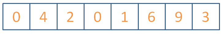
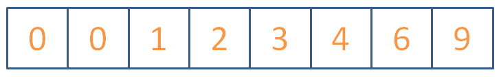
Use QuickSort to sort the following list of ints:
Click here for the steps the algorithm *could* take.
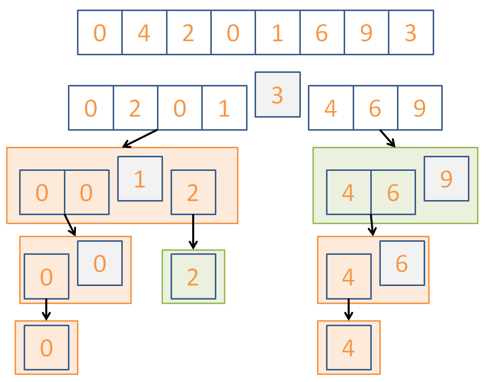
Here's a, perhaps more intuitive, implementation of quicksort that has an increased high space cost but illustrates the point:
  vector<int> quickSort (vector<int> arr) {
      // Base case: return current array if 1
      // element or fewer
      if (arr.size() <= 1) {return arr;}

      // Randomly choose a pivot
      int pivotChoice = (rand() % arr.size());
      int pivot = arr[pivotChoice];

      // We'll make 3 blank vectors: 1 that holds
      // all of the numbers less than the pivot,
      // 1 that holds all of the numbers greater,
      // and then 1 that just holds the pivot itself
      // for ease of concatenation
      vector<int> lesser, greater, pivotHolder;
      vector<int>::iterator it = arr.begin();
      pivotHolder.push_back(pivot);

      // Erase the pivot from the current vector
      arr.erase(it + pivotChoice);

      for (int i = 0; i < arr.size(); i++) {
          // Put remaining elements in their respective
          // greater or less than piles
          if (arr[i] < pivot) {
              lesser.push_back(arr[i]);
          } else {
              greater.push_back(arr[i]);
          }
      }

      // Recurse on the lesser and greater vectors,
      // and then concatenate their results with the
      // pivot in the center
      return concatVect(quickSort(lesser),
             concatVect(pivotHolder, quickSort(greater)));
  }

  int main () {
      int i[] = {0, 4, 2, 0, 1, 6, 9, 3};
      vector<int> v(i, i+8);
      v = quickSort(v);
      printIntVArr(v);
  }
Is QuickSort going to perform equally well every time it runs?
No! We can get really unlucky with pivot choices and divisions, trending towards O(n^2)
So what is the time complexity of QuickSort?
The average case is that it hits O(n*log(n)) because of its divide and conquer behavior.
There are a variety of improvements to this QuickSort algorithm that better its performance, including:
Perform a 3-way partitioning
When a sub list is small enough (typically around 9 items) use another sort like insertion sort, then recombine upwards.
Warning: QuickSort performs best when the elements are randomly distributed; a lack of unique values will actually slow it down!
There are some good QuickSort animations located here.
Now that you're accustomed to QuickSort, this won't be you in a job interview:

Practice
How about a couple of practice problems to round this all out?
The following examples show a starting list of ints, followed by several steps taken by a sorting algorithm. Identify which algorithm(s) are being applied!
  8, 6, 1, 2, 5, 0, 7, 3, 9, 4
  ====== BEGIN SORTING ======
  6, 8, 1, 2, 5, 0, 7, 3, 9, 4
  6, 1, 8, 2, 5, 0, 7, 3, 9, 4
  1, 6, 8, 2, 5, 0, 7, 3, 9, 4
  1, 6, 2, 8, 5, 0, 7, 3, 9, 4
  1, 2, 6, 8, 5, 0, 7, 3, 9, 4
  1, 2, 6, 8, 5, 0, 7, 3, 9, 4
  1, 2, 6, 5, 8, 0, 7, 3, 9, 4
  1, 2, 5, 6, 8, 0, 7, 3, 9, 4
  1, 2, 5, 6, 8, 0, 7, 3, 9, 4
  1, 2, 5, 6, 0, 8, 7, 3, 9, 4
  1, 2, 5, 0, 6, 8, 7, 3, 9, 4
  1, 2, 0, 5, 6, 8, 7, 3, 9, 4
  1, 0, 2, 5, 6, 8, 7, 3, 9, 4
How many *swaps* will BubbleSort make in sorting the following:
1, 2, 0, 3, 4
Which sorting algorithm will excel at sorting the following input? Which will degenerate toward quadratic time?
0, 0, 0, 0, 2, 2, 1, 1, 2, 2, 1, 1, 3, 3, 3, 3, 4, 4, 4, 4
Tree Basics
Hey, remember doubly linked lists?
Yeah me neither... well that's OK, here's a refresher:
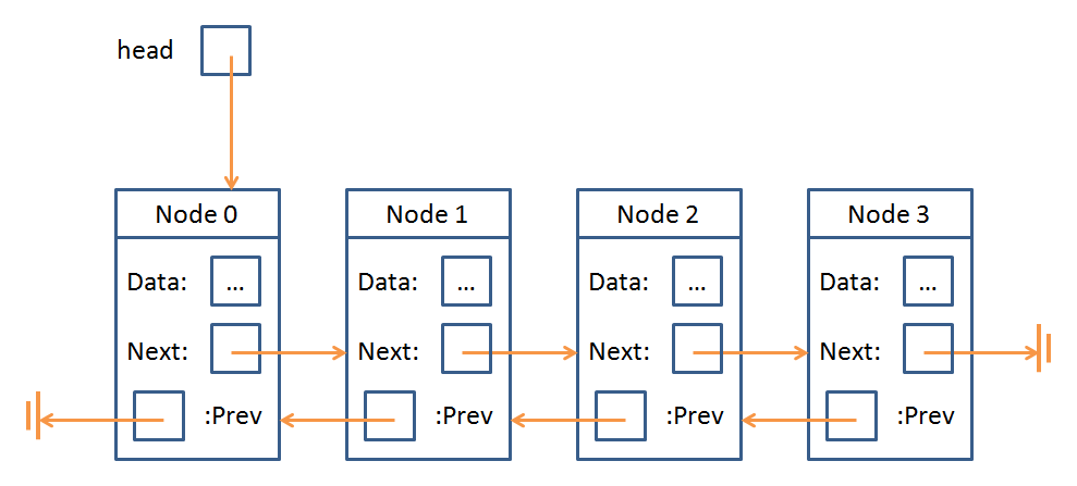
Double linked lists consisted of a sequence of nodes with data elements and pointers to the previous and next node in the sequence.
Indeed, the concept of a Node is something that Trees and Linked Lists have in common:
A Node is just an object that stores some data as well as a means of accessing other Nodes in the data structure.
The "means of accessing other Nodes" from a Node in a Linked List was to traverse it via prev and next; for Trees, it's only slightly more complicated.
Trees (in the general definition) possess Nodes with any number of "children," which are pointers to the next Node in the Tree.
Let's go over some definitions, see a Tree, and then run some code!
A Tree is yet another abstract data type consisting of data nodes arranged hierarchically, with a root node possessing some number of pointers (edges) to other children nodes, who in turn have their own children, etc.
There are two primary constraints for a Tree to be a... Tree: (1) no node's pointer (edge) points to the root, and (2) no two pointers point to the same node.
To formalize some of those definitions:
The root of a tree is a single node that has no inbound edges.
A leaf node is one that has no outbound edges.
An internal node has both inbound and outbound edges.
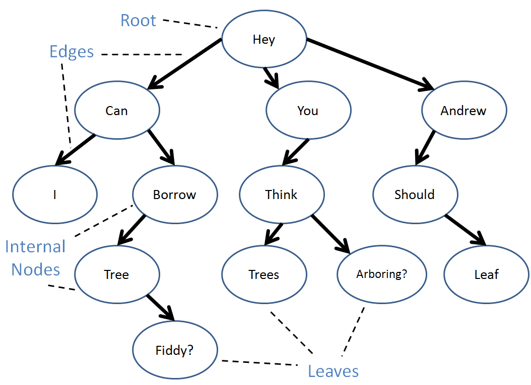
A tree can have duplicate values in its data nodes.
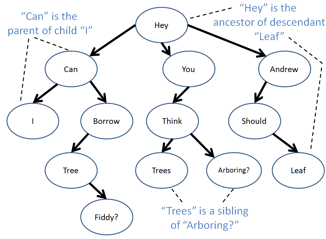
There are also a variety of relationships we can define between nodes:
An edge extends from a parent to a child with the arrow pointing to the child.
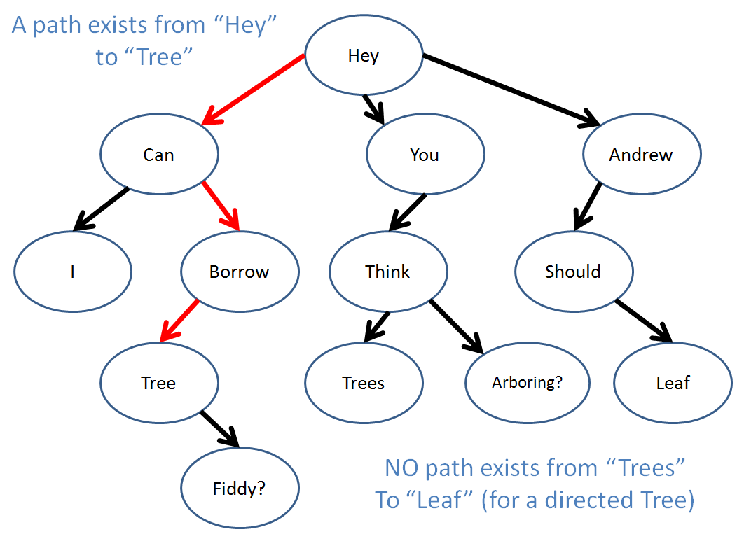
An path is any set of connected, directed edges.
A descendant of a node A is any node B with a directed path from A to B.
An ancestor of a node B is any node A with a directed path from A to B.
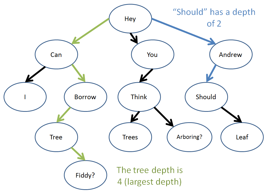
The depth of a node is equal to the number of edges along the path that separate it and the root.
The tree-depth a given tree is equal to maximum depth of any node in the tree.
Well, those are the tree basics! Let's look at some code now...
Tree Algorithms
I hope you liked recursion because trees were built for it! (or from it? any who...)
Let's start off with how we might construct a Node class:
  struct TreeNode {
      int data;
      TreeNode(int d) {data = d;}
      void addChild (TreeNode* c) {
          this->children.push_back(c);
      }
      vector<TreeNode*> children;
  };
Here, we have our TreeNode with an int data member and then an STL vector with TreeNode pointers to all of that TreeNode's children.
Let's reformat our tree from before with numerical values.
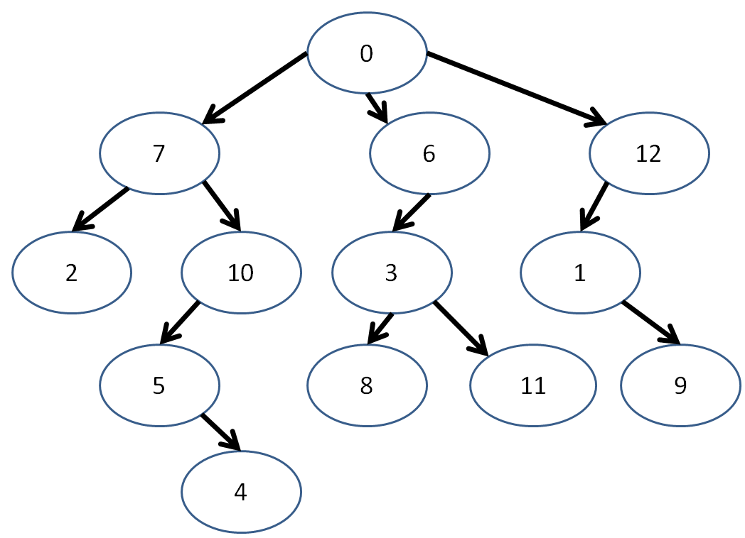
Now, let's say I wanted to create this tree using my new TreeNode class... since my numbers are conveniently in sequence, I can make a vector with them and then create the edges!
  int main () {
      vector<TreeNode> tree;
      int nodes = 13;

      // Create the TreeNodes in the tree
      for (int i = 0; i < 13; i++) {
          tree.push_back(TreeNode(i));
      }

      // Connect the nodes with edges!
      // (obviously there's a better way to do
      // this that we'll discuss next time)
      // [!] Left branch
      tree[0].addChild(&tree[7]);
      tree[7].addChild(&tree[2]);
      tree[7].addChild(&tree[10]);
      tree[10].addChild(&tree[5]);
      tree[5].addChild(&tree[4]);

      // [!] Middle branch
      tree[0].addChild(&tree[6]);
      tree[6].addChild(&tree[3]);
      tree[3].addChild(&tree[8]);
      tree[3].addChild(&tree[11]);

      // [!] Right branch
      tree[0].addChild(&tree[12]);
      tree[12].addChild(&tree[1]);
      tree[1].addChild(&tree[9]);

      // ...
  }
Now, before we dive head-first into Tree algorithms, we should always be on the lookout for these 4 test cases:
Does my algorithm work (read: not break) for an input nullptr?
Does my algorithm work for an input root node?
Does my algorithm work for an input interior node?
Does my algorithm work for an input leaf node?
Let's start off light with the following problem... which might look a little familiar:
  // Returns the maximum data node value in the
  // tree; expect no input nullptr
  int maxInTree (TreeNode* n) {
      // Set the current max to the input node's
      // data member
      int currentMax = n->data;

      // Find the max of each child's subtree
      for (int i = 0; i < n->children.size(); i++) {
          // Set currentMax equal to the max of
          // child i's subtree
          currentMax = max(currentMax, maxInTree(n->children[i]));
      }
      return currentMax;
  }
Not too bad... let's try one ourselves:
Modify your maxInTree function to implement treeDepth, a function that determines the tree depth of the input tree (TreeNode pointer).
  int treeDepth (TreeNode* n) {
      int currentMax = 0;
      for (int i = 0; i < n->children.size(); i++) {
          currentMax = ??? ;
      }
      return currentMax;
  }
Implement the nodesAtLevel function, which returns the number of nodes located at the depth specified.
  int nodesAtLevel (TreeNode* n, int level) {
      // Base case! Return when...
      if ( ??? ) {
          return ???;
      }

      // Iterate through every child
      int nodes = 0;
      for (int i = 0; i < n->children.size(); i++) {
          // [!] Add the number of nodes at the next level
          // if that's our target level! (hint: don't
          // need to use a conditional due to our base case)
          nodes += ???;
      }
      return nodes;
  }
Cool! How about a question to round things off?
Are all doubly linked lists also trees?
No! Linked lists allow for the possibility of cycles.
N-ary Trees
Whereas with the general definition of a tree allowed us to specify an arbitrary number of children for any node, there may be some benefits in restricting that number...
An n-ary tree is a tree in which each node can have at most n children.
Thus, a binary tree has nodes with at most 2 children, a trinary tree has nodes with at most 3 children... etc.
For the purposes of this discussion, we'll be examining binary trees.
Hey! Here comes one now!
"Hey... isn't that just the last example but with the right branch gone and a couple of numbers swi--"
It's 3:00am! Sue me!
Now, the Node structure that we define for binary trees might look a tiny bit different, just by convention because we like to define "left" and "right" children.
  struct BinTreeNode {
      int data;
      BinTreeNode* left;
      BinTreeNode* right;
      BinTreeNode(int d) {
          data = d;
          left = nullptr;
          right = nullptr;
      }
  };
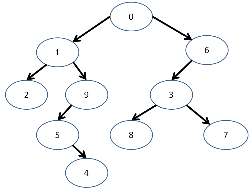
Again representing our example from above:
  int main () {
      vector<BinTreeNode> tree;
      int nodes = 10;

      // Create the TreeNodes in the tree
      for (int i = 0; i < nodes; i++) {
          tree.push_back(BinTreeNode(i));
      }

      // Connect the nodes with edges!
      // (obviously there's a better way to do
      // this that we'll discuss next time)
      // [!] Left branch
      tree[0].left = &tree[1];
      tree[1].left = &tree[2];
      tree[1].right = &tree[9];
      tree[9].left = &tree[5];
      tree[5].right = &tree[4];

      // [!] Right branch
      tree[0].right = &tree[6];
      tree[6].left = &tree[3];
      tree[3].left = &tree[8];
      tree[3].right = &tree[7];

      // ...
  }
Let's look at some neat properties of binary trees.
Tree Traversal
Tree traversal determines the order in which we visit each node in a tree, starting at some node (usually the root).
Traversal strategies are defined recursively, in terms of the current node, its left child, and its right child.
There are three primary traversal strategies under the heading of "Depth first" which we'll talk about later:
Pre-order Traversal
The preorder traversal strategy follows these steps:
Visit the current node (base case)
Visit the left subtree (recursive case)
Visit the right subtree (recursive case)
The definition of "visit" will depend on your application. For the moment, let's consider our application to be simply to print out the data at each Node in a given order.
  // Prints the data in each node using
  // the preorder traversal strategy
  void preorderPrint (BinTreeNode* n) {
      if (n == nullptr) {return;}
      cout << n->data << endl;
      preorderPrint(n->left);
      preorderPrint(n->right);
  }
Preorder traversal looks like this:
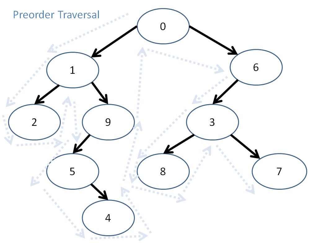
So, here, preorder traversal prints out: 0, 1, 2, 9, 5, 4, 6, 3, 8, 7
Post-order Traversal
The postorder traversal strategy follows these steps:
Visit the left subtree (recursive case)
Visit the right subtree (recursive case)
Visit the current node (base case)
NOTE: This means, even though we might "pass through" a node, we don't print it until its left and right subtrees have been processed!
Here is the postorderPrint function:
  void postorderPrint (BinTreeNode* n) {
      if (n == nullptr) {return;}
      postorderPrint(n->left);
      postorderPrint(n->right);
      cout << n->data << endl;
  }
So, what will the postorder traversal of our tree print out?
The postorder traversal prints...
2, 4, 5, 9, 1, 8, 7, 3, 6, 0
In-order Traversal
The inorder traversal strategy follows these steps:
Visit the left subtree (recursive case)
Visit the current node (base case)
Visit the right subtree (recursive case)
For completion, here's that in code form:
  void inorderPrint (BinTreeNode* n) {
      if (n == nullptr) {return;}
      inorderPrint(n->left);
      cout << n->data << endl;
      inorderPrint(n->right);
  }
Applications for Binary Trees
We've already discussed one of the most prevalent applications for binary trees: binary search.
A binary search tree is a binary tree in which all elements in the left subtree of a node are less than the data member of that node, and all elements of the right subtree are greater than the data member of that node.
Some other constraints for binary search trees is that there must be no duplicate nodes, and the left and right subtrees of each node must also be a binary search tree.
Let's revise our ongoing example:
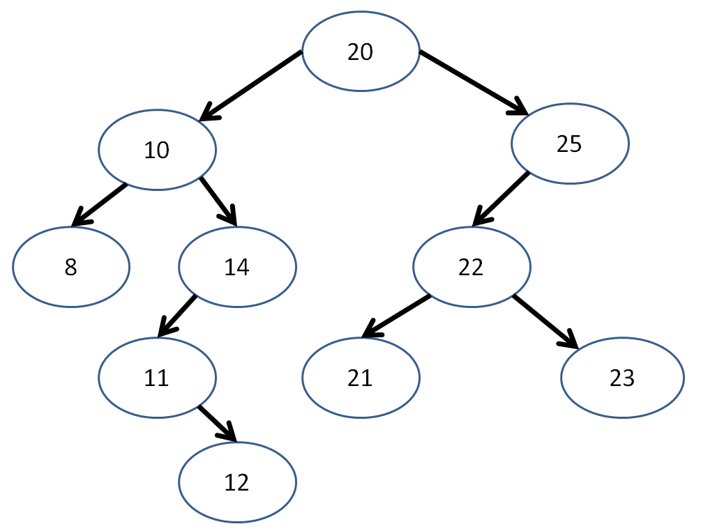
We observe that, for each node, the left subtree contains data elements strictly less than the data element of the subtree root, and vice versa for the right subtrees.
Now, binary search becomes a trivial algorithm:
  bool binarySearch (BinTreeNode* n, int query) {
      if (n == nullptr) {return false;}
      if (n->data == query) {return true;}
      else if (query < n->data) {
          return binarySearch(n->left, query);
      } else {
        return binarySearch(n->right, query);
      }
  }
Practice Problems
Provide two binary trees that could elicit the preorder traversal print out: 5, 3, 1, 2, 0
Is it possible for a binary search tree to have the postorder traversal print out of: 12, 18, 14, 21, 20, 17
No! The 18 wedged between the 12 and 14 implies that a number greater than the root (which we know must be 17 because it was printed last) existed on the side intended to be less than the root.